Understanding Emissions Impact in Microgrid Projects
Adaptive Intelligence Over Predictive Accuracy

Why Emissions Calculations Matter More Than Ever
As organizations increasingly commit to carbon reduction goals, understanding the true emissions impact of energy infrastructure projects has become both a regulatory requirement and a competitive necessity. Yet when it comes to microgrid projects, calculating emissions impact presents unique challenges that traditional grid-connected systems simply don’t face.
Consider this: a hospital installing a microgrid might reduce its carbon footprint by 30% during normal grid-connected operations, but what happens during the inevitable power outages when diesel generators kick in? How do we account for the solar panels that sometimes export excess energy to the grid? These nuanced scenarios require a sophisticated approach that goes beyond simple emissions factors.
At ProtoGen, we’ve developed a comprehensive methodology that addresses these complexities head-on. This paper walks through our approach, explains the critical decisions that shape emissions calculations, and provides practical guidance for anyone working with distributed energy systems.
The Foundation: Two Categories of Emissions
Understanding microgrid emissions starts with recognizing that energy flows in two distinct directions, each creating different types of environmental impact. Think of it like a conversation between your facility and the broader electrical grid – sometimes you’re listening (consuming power), sometimes you’re speaking (generating and potentially exporting power), and occasionally you’re having a private conversation (operating independently during outages).
Local Electricity-Generating Emissions
Local emissions come from any generation equipment operating within your facility boundaries. This includes diesel generators, natural gas turbines, fuel cells, and any other equipment that burns fuel or releases emissions during the power generation process. These emissions include not just carbon dioxide (CO₂), but also methane (CH₄), nitrous oxide (N₂O), and particulate matter (PM₂.₅).
The key insight here is control and timing. Unlike grid emissions, which happen regardless of your facility’s actions, local emissions are directly under your operational control. When your backup generator runs, those emissions are entirely attributable to your energy decisions.
Indirect Emissions from Grid Consumption
Grid emissions represent the environmental impact of the electricity you purchase from or export to the broader electrical system. These emissions don’t occur at your facility, but they happen because of your energy consumption patterns. When you reduce your grid purchases by running your own solar panels, you’re theoretically reducing the need for grid-scale generation somewhere else in the system.
The challenge lies in determining exactly which power plants are affected by your actions. When you flip a light switch, you’re not directly connected to a specific power plant – you’re tapping into a vast, interconnected system where supply and demand are constantly balanced by system operators.
Challenges In Microgrid Emissions Calculations
The Outage Dependency Problem
Here’s where microgrid emissions calculations become particularly complex: most distributed generation resources in a microgrid context only operate during grid outages. This creates a fundamental timing dependency that doesn’t exist in traditional grid-connected systems.
Imagine trying to calculate the emissions impact of a backup generator that might run for four hours twice a year, or for forty hours during a major storm. The total emissions depend entirely on outage frequency, duration, and timing – variables that are inherently unpredictable. This uncertainty means that emissions calculations often rely on probabilistic estimates rather than deterministic values.
The customer becomes a critical partner in this process, as they often have the best historical data and institutional knowledge about outage patterns. A hospital in a hurricane-prone region will have very different outage expectations than a manufacturing facility in an area with reliable grid service.
The Existing Generator Complication
Many facilities considering microgrids already operate backup generators, which adds another layer of complexity to emissions calculations. When a microgrid is installed, these existing generators typically don’t disappear – they often transition into secondary or supplementary roles within the new system architecture.
This transition raises important questions: If a facility previously relied entirely on a diesel generator during outages but now uses a combination of solar, battery storage, and the same diesel generator, how do we calculate the net emissions change? The generator might run less frequently but potentially for longer durations. The load being supported might increase because the facility can now maintain more operations during outages.
These scenarios require careful baseline establishment and clear assumptions about operational changes. The emissions impact isn’t just about the new equipment – it’s about how the entire energy system evolves.
The Marginal Emissions Challenge
Grid emissions calculations face a fundamental conceptual hurdle: understanding the difference between average and marginal emissions. This distinction is crucial but often misunderstood, even among energy professionals.
Average emissions represent the total emissions from all power plants divided by total electricity generation – essentially the “average carbon intensity” of the grid. Marginal emissions, however, represent the emissions from the specific power plant that would increase or decrease output in response to your facility’s changing electricity demand.
Here’s why this matters: if you reduce your electricity consumption by 100 kWh at 2 PM on a sunny Tuesday, that reduction might allow a natural gas peaker plant to reduce output, avoiding the emissions associated with burning natural gas. But if you make the same 100 kWh reduction at 3 AM on a calm Sunday, it might allow a wind farm to reduce output, avoiding essentially zero emissions.
This dynamic nature of marginal emissions means that the timing of your energy actions dramatically affects their environmental impact. A battery storage system that charges during high-renewable periods and discharges during high-carbon periods can have significantly greater emissions benefits than the same system operating on a simple time-of-use schedule.
The complexity of this marginal emissions signal is thoroughly explored in an excellent analysis by Electricity Maps, which provides essential background for understanding why traditional average emissions approaches fall short in dynamic grid environments.
The PV Export Uncertainty
Solar photovoltaic systems present their own unique challenges, particularly when they generate more electricity than the facility consumes. What’s the emissions impact of exporting excess solar energy to the grid?
The conceptual approach is straightforward: exported solar energy should displace grid generation, creating emissions benefits similar to reduced consumption. However, the practical implementation raises complex questions about timing, grid constraints, and system operations.
When your solar panels export 50 kWh to the grid at noon, does that energy directly displace fossil fuel generation, or does it simply reduce the output of other renewable sources that were already operating? The answer depends on grid conditions, transmission constraints, and the specific generation mix operating at that moment.
ProtoGen’s approach treats PV exports as equivalent to load reductions, using the same marginal emissions factors. This methodology provides consistency and reflects the general principle that additional clean energy displaces marginal generation, but we acknowledge this is an area where industry practices continue to evolve.
ProtoGen's Methodology: A Step-By-Step Approach
Local Emissions Calculation Framework
Our approach to local emissions begins with a fundamental choice: we calculate based on electricity generated rather than fuel consumed. This approach aligns with how facilities typically monitor and optimize their energy systems, and it directly connects to the services the generation equipment provides.
The core calculation follows EPA guidance and can be expressed as:
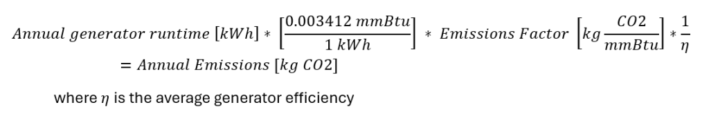
Let’s break this down step by step:
Step 1: Determine Generator Runtime | We start with the expected annual electricity generation from on-site equipment, measured in kilowatt-hours. This figure comes from operational projections based on expected outage patterns, equipment sizing, and load requirements during islanded operation.
Step 2: Convert to Energy Content | The conversion factor 0.003412 mmBtu per kWh translates electrical output back to the thermal energy content. This step is necessary because EPA emissions factors are expressed in terms of fuel energy content rather than electrical output.
Step 3: Apply Emissions Factors | EPA provides standardized emissions factors for different fuel types, expressed as kilograms of CO₂ equivalent per million British thermal units (mmBtu) of fuel energy. These factors account for the carbon content of different fuels and the stoichiometry of combustion.
Step 4: Adjust for Efficiency | The efficiency factor (η) accounts for the fact that generators convert only a portion of fuel energy into electricity. A generator that’s 35% efficient requires more fuel – and produces more emissions – per kWh of electricity than a 40% efficient unit.
This methodology provides a transparent, reproducible approach that facility operators can understand and verify against their operational experience.
Grid Marginal Emissions Framework
Calculating the emissions impact of changes in grid electricity consumption requires a different approach, one that accounts for the dynamic nature of electricity systems and the specific timing of energy transactions.
The fundamental equation is:
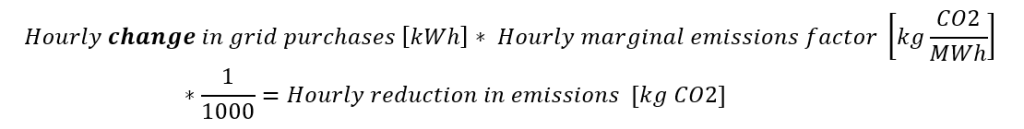
To better understand marginal emissions data, we rely on specialized data providers like WattTime, who use sophisticated modeling to estimate the marginal emissions intensity of electricity grids in real-time. This organization analyze generation dispatch data, fuel prices, transmission constraints, and system operations to determine which power plants are most likely to respond to changes in electricity demand.
Hourly time resolution or sometimes called hourly granularity, is critical because marginal emissions can vary dramatically throughout the day. During periods of high renewable generation, marginal emissions might be very low or even negative (indicating that reduced consumption might actually increase emissions by forcing renewable sources offline). During peak demand periods, marginal emissions are typically higher as less efficient “peaker” plants come online.
When calculating the benefits of solar PV exports, we use the same marginal emissions factors applied to consumption reductions. This approach assumes that exported solar energy displaces marginal grid generation, creating emissions benefits equivalent to reducing consumption by the same amount.
Integrating the Components
The final step brings together local generation emissions and grid interaction benefits into a comprehensive picture:

This equation captures the full environmental story: how much your facility reduces grid-related emissions through changed consumption patterns and clean energy exports, minus any emissions created by your own generation equipment.
The Future Of Intelligent Emissions Optimization
While the methodology described above focuses on planning, design, and reporting applications, the real opportunity lies in moving beyond static calculations toward dynamic, intelligent operational optimization. Imagine a microgrid controller that doesn’t just follow predetermined schedules, but continuously optimizes between multiple objectives including time-of-use pricing tariffs and real-time grid emissions signals.
This vision represents a fundamental shift from asking “What will our emissions impact be?” to enabling systems that ask “How should we operate right now to achieve our desired balance between cost savings and emissions reduction?”
Real-Time Optimization Architecture
Consider a hospital microgrid equipped with solar panels, battery storage, and backup generators, managed by an intelligent controller that receives live data streams including electricity pricing, marginal emissions factors, weather forecasts, and facility load predictions. Rather than operating on fixed schedules, this system continuously recalculates optimal dispatch decisions based on current conditions and user-defined priorities.
When grid emissions are high due to fossil fuel peaker plants operating, the controller prioritizes battery discharge and on-site solar generation, even if electricity prices are relatively low. During periods of abundant renewable generation when marginal emissions approach zero, the system might choose to charge batteries from grid power despite slightly higher costs, knowing that this stored energy can displace higher-carbon generation later in the day.
The user sets high-level objectives – perhaps 70% weight on cost optimization and 30% on emissions reduction – and the intelligent controller translates these preferences into thousands of operational decisions throughout the year. Each decision considers not just immediate conditions, but also forecasted changes in pricing, emissions, weather, and facility needs.
The Implementation Advantage
Here’s a crucial insight that emerges from working with these systems: implementing intelligent operational control may actually be easier than accurately modeling long-term emissions outcomes. While projecting grid evolution over a 20-year project lifetime involves enormous uncertainty about technology deployment, regulatory changes, and market structures, responding to current conditions requires only reliable real-time data and robust optimization algorithms.
This suggests a path forward that emphasizes adaptive intelligence over predictive accuracy. Rather than trying to perfectly model future grid conditions, we can build systems that continuously adjust to actual conditions as they evolve. The microgrid controller doesn’t need to know what the grid will look like in 2040 – it just needs to optimize effectively for whatever conditions exist at any given moment.
Integration with Existing Infrastructure
This intelligent optimization approach integrates naturally with existing microgrid components and control systems. Modern inverters, battery management systems, and generator controllers already communicate through standardized protocols. The intelligent layer adds decision-making capabilities that coordinate these components toward user-defined objectives rather than simple operational rules.
The key technological components already exist: reliable marginal emissions data from services like WattTime, sophisticated optimization algorithms from the research community, and communication protocols that enable real-time coordination of distributed energy resources. The challenge lies in integrating these components into reliable, user-friendly systems that facility operators can understand and trust.
Building Trust Through Transparency
For intelligent emissions optimization to gain widespread adoption, users need to understand and trust the system’s decision-making process. This means providing clear explanations of why the controller made specific choices, how those choices align with user priorities, and what trade-offs were considered.
A hospital energy manager should be able to review yesterday’s operations and understand why the battery charged at 2 PM (low grid emissions) and discharged at 7 PM (high grid emissions), how much money was saved versus a simple time-of-use strategy, and what the emissions impact was. This transparency builds confidence and enables users to refine their objective settings based on actual outcomes.
This vision of intelligent operational optimization represents the next frontier in microgrid development – moving beyond static planning tools toward dynamic systems that continuously optimize environmental and economic performance based on real-world conditions.
Implementation Considerations and Best Practices
Data Alignment and Quality Control
One of the most critical but often overlooked aspects of emissions calculations is ensuring that all data sources reference the same time periods. Microgrid optimization typically involves complex interactions between solar irradiance, outdoor temperature, facility electricity consumption, and regional marginal emissions. If for example the solar dataset is from 2022 but the emissions data is from 2021, or if time zones don’t match, the resulting analysis can be significantly flawed.
Think of it like trying to conduct a symphony where the musicians are reading sheet music from different compositions. Each dataset might be accurate individually, but the combination produces meaningless results. This data alignment challenge becomes particularly acute when working with Mixed Integer Linear Programming (MILP) optimization tools like Xendee or ReOpt, which require precisely synchronized inputs to produce meaningful outcomes.
Emissions Analysis Insights: When Timing and Scale Matters
When data alignment is properly executed, the resulting emissions analysis reveals fascinating patterns that emphasize why precise timing matters for carbon impact assessments. Our analysis of PJM grid emissions data demonstrates several critical insights through various patterns that could directly influence microgrid design and operational strategies.
Temporal Emissions Patterns Drive Solar Value
Grid emissions exhibit distinct temporal patterns that create windows of opportunity for carbon reduction. The graphs below (Figure 1) reveal characteristic peaks during January, July, and December – periods when heating and cooling demand require utilities to deploy higher-emission peaking generation. Yellow areas show times when the electric grid produces more CO2 per kWh, while dark purple shows cleaner periods.
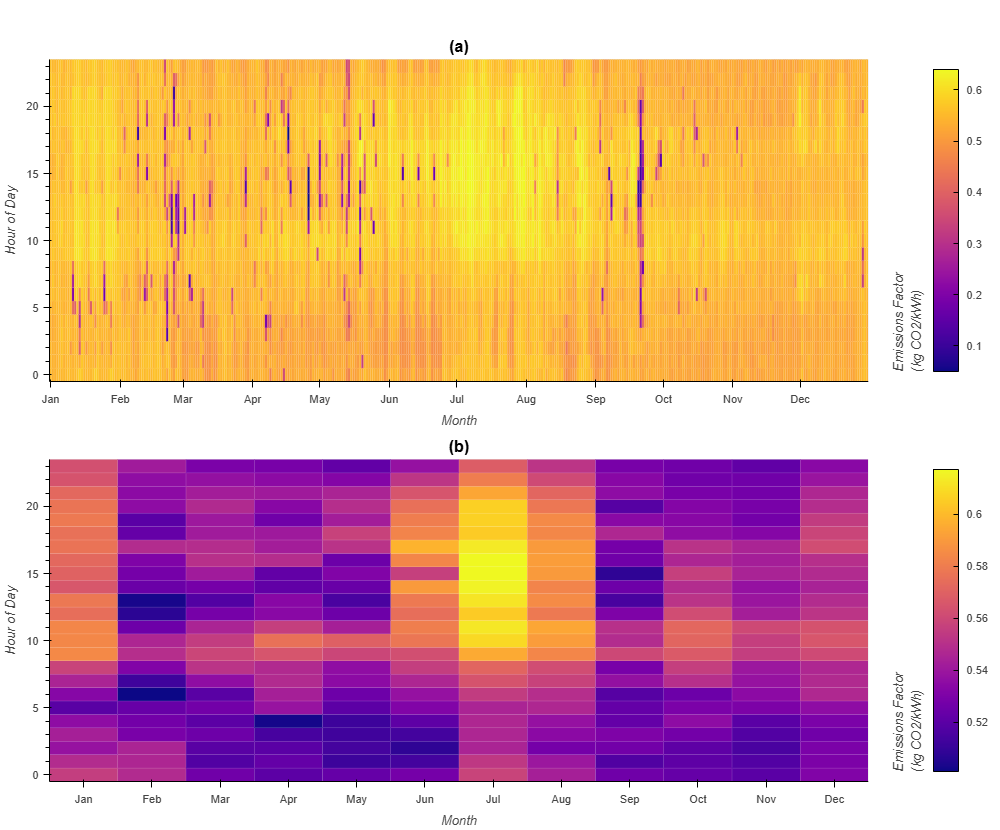
Figure 1: PJM Daily Emissions Factor Heatmaps showing (a) Day of Year vs. Hour and (b) Month vs. Hour
Daily patterns show elevated emissions around 10 AM, coinciding with commercial demand ramp-up before solar production peaks. These patterns create a left-skewed distribution where most hours have relatively high emissions (0.55-0.65 kg CO₂/kWh), but occasional periods of very low emissions occur when renewables dominate the grid mix (see Figure 2). The many dots below the boxes represent hours when wind and solar significantly reduces grid emissions, creating optimal timing for solar energy deployment.
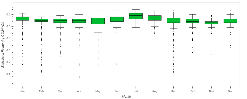
Figure 2: PJM Monthly Emissions Factor Distribution
System Sizing Creates Compounding Benefits
Comparing 75 kW versus 125 kW solar installations reveal that larger systems provide disproportionate emissions benefits.
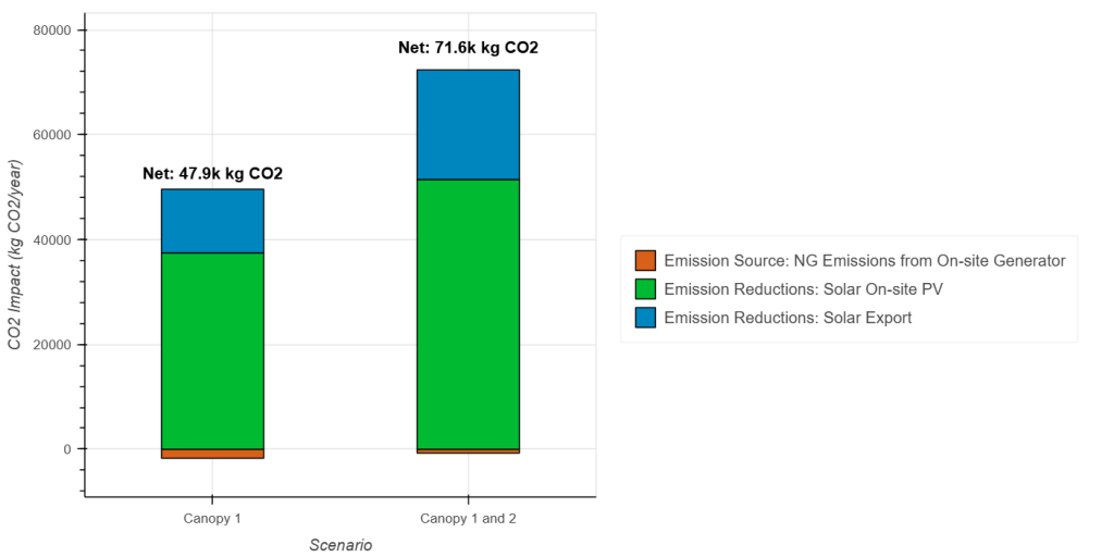
Figure 3: Annual CO2 Impact: Emission Reductions vs. Generator Emissions
The annual analysis (Figure 3) shows not only increased behind-the-meter reductions and solar exports from the larger array, but also reduced generator emissions – demonstrating how proper solar sizing can minimize backup generation needs while maximizing grid interaction benefits. Green and blue sections show CO2 reductions from solar, while orange shows emissions from backup generators during an outage. The 125 kW system delivers 71,600 kg of net CO2 reductions compared to 47,900 kg for the 75 kW system – a 49.5% improvement despite only a 67% increase in capacity.
Grid Outages Reshape the Carbon Equation
Perhaps most revealing is the impact of grid outages on emissions profiles. As shown in Figure 4, the purple dashed line marks when the grid outage began (July 14th), dramatically changing the emissions patterns. The stark contrast between pre- and post-outage periods illustrates how a single event can fundamentally alter a microgrid’s carbon impact profile. After the outage, orange spikes show backup generator emissions while green/blue reductions disappear during non-solar hours. During outage periods, generator emissions drop significantly for the larger PV array as solar and backup systems operate more efficiently when supporting critical loads only.
(a)
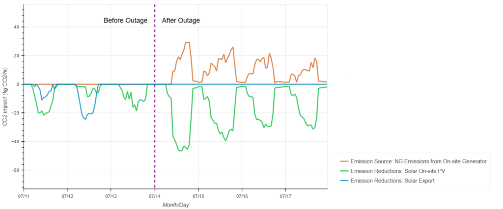
(b)
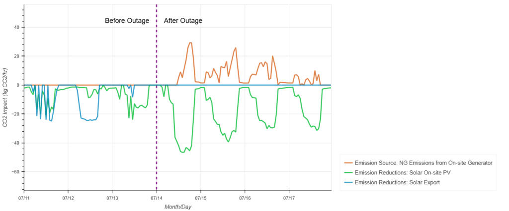
Figure 4: Weekly CO2 Emissions Impact during Grid Outage for (a) 75 kW PV array and (b) 125 kW PV array
However, this comes at the cost of zero solar exports, eliminating the opportunity to displace grid emissions for other customers. This trade-off highlights a fundamental tension in resilient microgrid design: optimizing carbon impact during normal operations versus maintaining essential services during emergencies.
These insights demonstrate why synchronized, high-quality data is essential – the complex interplay between solar production, building loads, grid emissions, and backup generation reveals optimization opportunities that are only visible when all data sources are properly aligned and analyzed together.
Managing Uncertainty and Sensitivity Analysis
Given the inherent uncertainties in outage projections, marginal emissions factors, and operational assumptions, robust emissions calculations should include sensitivity analysis. How much do the results change if outages are twice as frequent as expected? What if marginal emissions factors shift due to changing grid composition?
These sensitivity analyses help stakeholders understand the range of possible outcomes and make informed decisions about the relative importance of emissions benefits versus other project drivers like resilience or cost savings.
Long-Term Projections and Grid Evolution
One of the most significant gaps in current emissions calculation methods involves projecting impacts over a project’s operational lifetime. The electricity grid is changing rapidly, with increasing renewable penetration, changing dispatch patterns, and evolving regulations. A microgrid installed today will operate in a very different grid environment in 2040 than it does in 2025.
Research organizations like NREL are developing tools like Cambium to address these long-term projection challenges, but these methods are not yet widely adopted in commercial practice. This represents an important area for continued development and standardization across the industry.
Building Better Decisions Through Better Analysis
Accurate emissions calculations serve multiple critical functions in microgrid development. They support regulatory compliance, inform carbon accounting and sustainability reporting, enable meaningful comparisons between project alternatives, and help organizations make decisions aligned with their environmental commitments.
The methodology outlined here represents ProtoGen’s current best practice, developed through extensive project experience and ongoing research collaboration. However, we recognize that this field continues to evolve as grid systems become more complex, data sources improve, and regulatory frameworks develop.
The key insight for anyone working with distributed energy systems is that emissions calculations are not just technical exercises. They are decision making tools that shape how we design, operate, and value energy infrastructure. Getting them right requires not just technical accuracy, but also clear communication about assumptions, uncertainties, and limitations.
As the energy market continues to evolve, the demand for sophisticated, transparent, and actionable emissions analysis will only increase. Organizations that invest in developing these capabilities now will be better positioned to navigate the complex energy landscape ahead.
For more information about ProtoGen’s approach to microgrid development and emissions analysis, contact our technical team.